波形尖灭

波形尖灭#


波形尖灭是指在信号首尾施加平滑衰减窗函数,使振幅在两端平滑过渡至零,从而减少因信号截断引起的频谱泄漏。

设原始信号为 \(x(j)\)、窗函数为 \(w(j)\),则尖灭后的信号可表示为:

\[ x'(j) = w(j)*x(j), \]

其中 \(w(j)\) 在信号首尾逐渐从 0 过渡到 1,并在中间区域保持为 1,实现波形的尖灭。

下图比较了两种常用的尖灭窗:余弦窗 (cosine) 与 Hanning 窗 (hann)。本示例中,两端各 5% 长度用于平滑渐入/渐出,中间部分保持幅度 1。

Hide code cell source

import numpy as np
import matplotlib.pyplot as plt
from obspy.signal.invsim import cosine_taper  # ObsPy 余弦尖灭

# 参数设置
npts = 1000
p = 0.05  # 两端 5%

# 余弦尖灭窗
win_cos = cosine_taper(npts, p=p)

# Hanning 窗(构造两端平滑、中间平坦)
win_han = np.ones(npts)
edge = int(p * npts)
han_full = np.hanning(2 * edge)
win_han[:edge] = han_full[:edge]
win_han[-edge:] = han_full[-edge:]

x = np.linspace(0, 1, npts)
plt.figure(figsize=(9, 4))
plt.plot(x, win_cos, 'r-', lw=2, label=f'Cosine (p={p})')
plt.plot(x, win_han, 'b--', lw=2, label=f'Hanning (p={p})')
plt.xlabel('Normalized Time')
plt.ylabel('Amplitude')
plt.title('Cosine vs Hanning Taper Windows')
plt.legend()
plt.show()
---------------------------------------------------------------------------
ModuleNotFoundError                       Traceback (most recent call last)
Cell In[1], line 3
      1 import numpy as np
      2 import matplotlib.pyplot as plt
----> 3 from obspy.signal.invsim import cosine_taper  # ObsPy 余弦尖灭
      5 # 参数设置
      6 npts = 1000

File ~/micromamba/envs/seismo-learn/lib/python3.13/site-packages/obspy/__init__.py:44
     41     msg = ('pkg_resources is deprecated as an API')
     42     warnings.filterwarnings(
     43         'ignore', message=msg, category=DeprecationWarning, module='obspy')
---> 44     from obspy.core.utcdatetime import UTCDateTime  # NOQA
     45 from obspy.core.util import _get_version_string
     46 __version__ = _get_version_string(abbrev=10)

File ~/micromamba/envs/seismo-learn/lib/python3.13/site-packages/obspy/core/__init__.py:120
     12 """
     13 obspy.core - Core classes of ObsPy
     14 ==================================
   (...)    117 .. _NumPy: http://www.numpy.org
    118 """
    119 # don't change order
--> 120 from obspy.core.utcdatetime import UTCDateTime  # NOQA
    121 from obspy.core.util.attribdict import AttribDict  # NOQA
    122 from obspy.core.trace import Stats, Trace  # NOQA

File ~/micromamba/envs/seismo-learn/lib/python3.13/site-packages/obspy/core/utcdatetime.py:21
     18 import warnings
     20 import numpy as np
---> 21 from obspy.core.util.deprecation_helpers import ObsPyDeprecationWarning
     24 # based on https://www.myintervals.com/blog/2009/05/20/iso-8601, w/ week 53 fix
     25 _ISO8601_REGEX = re.compile(r"""
     26     ^
     27     ([\+-]?\d{4}(?!\d{2}\b))
   (...)     40     $
     41     """, re.VERBOSE)

File ~/micromamba/envs/seismo-learn/lib/python3.13/site-packages/obspy/core/util/__init__.py:22
     20 # import order matters - NamedTemporaryFile must be one of the first!
     21 from obspy.core.util.attribdict import AttribDict
---> 22 from obspy.core.util.base import (ALL_MODULES, DEFAULT_MODULES,
     23                                   NATIVE_BYTEORDER, NETWORK_MODULES,
     24                                   NamedTemporaryFile, _read_from_plugin,
     25                                   create_empty_data_chunk, get_example_file,
     26                                   get_script_dir_name, MATPLOTLIB_VERSION,
     27                                   SCIPY_VERSION, NUMPY_VERSION,
     28                                   CARTOPY_VERSION, CatchAndAssertWarnings)
     29 from obspy.core.util.misc import (BAND_CODE, CatchOutput, complexify_string,
     30                                   guess_delta, score_at_percentile,
     31                                   to_int_or_zero, SuppressOutput)
     32 from obspy.core.util.obspy_types import (ComplexWithUncertainties, Enum,
     33                                          FloatWithUncertainties)

File ~/micromamba/envs/seismo-learn/lib/python3.13/site-packages/obspy/core/util/base.py:26
     23 from pathlib import PurePath
     25 import numpy as np
---> 26 import pkg_resources
     27 from pkg_resources import get_entry_info, iter_entry_points
     29 from obspy.core.util.misc import to_int_or_zero, buffered_load_entry_point

ModuleNotFoundError: No module named 'pkg_resources'

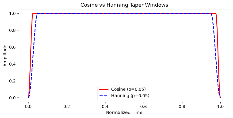
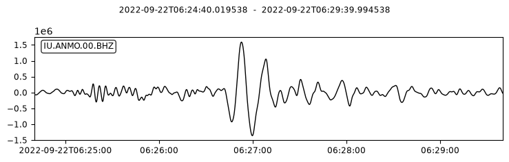
我们以前一节使用的 2022 年 9 月 22 日墨西哥 Mw 6.8 地震在 ANMO 台站的波形为例。

from obspy import UTCDateTime
from obspy.clients.fdsn import Client
import matplotlib.pyplot as plt

client = Client("IRIS") 

# 下载 2022 年墨西哥 Mw 6.8 级地震在 ANMO 台站的波形数据(选择 400–700 s 时间窗)
origin_time = UTCDateTime("2022-09-22T06:18:00")
starttime = origin_time + 400
endtime = origin_time + 700
st = client.get_waveforms(
    network="IU",
    station="ANMO", 
    location="00", 
    channel="BHZ",
    starttime=starttime, 
    endtime=endtime,
)
st.plot();

进行尖灭处理之前,通常先进行去均值、去线性趋势。

tr = st[0]

# 去均值 + 去趋势
tr.detrend("demean")
tr.detrend("linear")

tr_origin = tr.copy()   # 备份原始波形

波形尖灭可使用 ObsPy 的 obspy.core.trace.Trace.taper() 实现。

在实际数据处理中,常使用 5% 的 Hanning 窗(taper 中的 type 参数默认即为 hann)。 
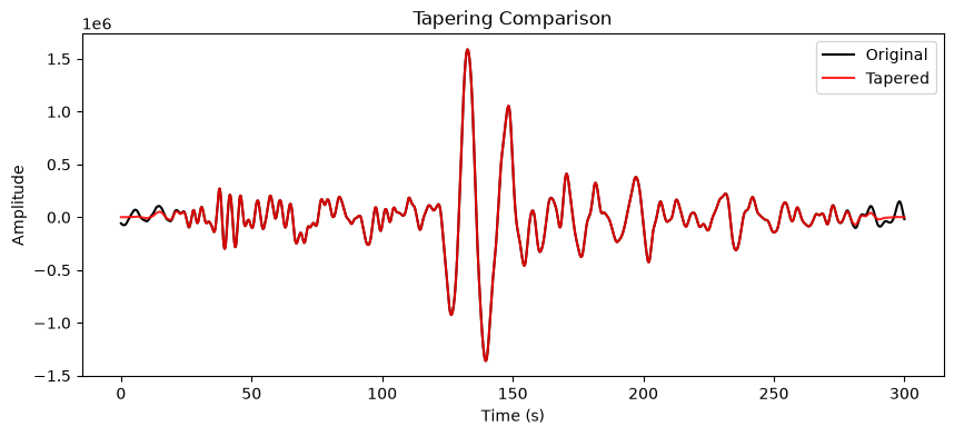
本例中为了使尖灭的效果更明显,使用 10% 的 Hanning 窗(max_percentage=0.1):

tr.taper(max_percentage=0.1, type="hann")

下图演示了尖灭操作的效果:黑色和红色分别为尖灭操作前后的波形。可以看到,原始波形(黑) 在截断处存在“硬边界”,而尖灭后(红)两端平滑过渡至零,能有效抑制频谱泄漏。

plt.figure(figsize = (10, 4))
plt.plot(tr_origin.times(), tr_origin.data, 'k-', label='Original')
plt.plot(tr.times(), tr.data, 'r-', label='Tapered', alpha=0.85)
plt.xlabel('Time (s)')
plt.ylabel('Amplitude')
plt.title('Tapering Comparison')
plt.legend()
plt.show()