本节贡献者: 田冬冬、姚家园
最近更新日期: 2022-07-31
预计花费时间: 15 分钟
在获取地震目录之后,通常还需要对地震目录做一些简单的绘图和分析。这一节演示如何 绘制最简单的地震深度直方图、地震震级直方图以及震级-频次关系图。
首先,需要把地震目录准备好。这里我们选择下载 2000–2010 年间震级大于 4.8 级, 震源深度大于 50 km 的地震。这一地震目录中共计约 7000 个地震:
from obspy.clients.fdsn import Client

client = Client("USGS")
cat = client.get_events(
    starttime="2000-01-01",
    endtime="2010-01-01",
    minmagnitude=4.8,
    mindepth=50,
)
print(cat)
6982 Event(s) in Catalog:
2009-12-31T17:42:15.960000Z | -19.747, -177.753 | 5.4 mwc | manual
2009-12-31T09:06:01.250000Z | -7.499, +127.930 | 5.1 mb | manual
...
2000-01-02T12:14:39.090000Z | -17.943, -178.476 | 5.5 mwc | manual
2000-01-01T05:24:35.290000Z | +36.874, +69.947 | 5.1 mwc | manual
To see all events call 'print(CatalogObject.__str__(print_all=True))'
为了进一步对数据做处理以及绘图,我们还需要导入 NumPy 和 Matplotlib 模块:
import matplotlib.pyplot as plt
import numpy as np
地震深度分布直方图
为了绘制地震深度直方图,我们先从地震目录中提取出地震深度信息,并保存到数组 depth 中。
需要注意的是,ObsPy 的地震目录中地震深度的单位为 m,所以需要除以 1000.0 将深度单位
转换为 km。
depth = np.array([event.origins[0].depth / 1000 for event in cat])我们可以使用 Matplotlib 的 ~matplotlib.axes.Axes.hist() 函数绘制直方图:
这里我们设置的直方的最小值为 50,最大值 700,间隔为 10,同时设置了 Y 轴以对数方式显示。
从图中可以明显看到地震深度随着深度的变化:
fig, ax = plt.subplots()
ax.hist(depth, bins=np.arange(50, 700, 10), log=True)
ax.set_xlabel("Depth (km)")
ax.set_ylabel("Number of earthquakes")
plt.show()
地震震级直方图
同理,从地震目录中提取出地震震级信息,保存到数组 mag 中并绘图。从图中可以明显看到,
震级越小地震数目越多:
mag = np.array([event.magnitudes[0].mag for event in cat])

fig, ax = plt.subplots()
ax.hist(mag, bins=np.arange(4.5, 8, 0.1))
ax.set_xlabel("Magnitude")
ax.set_ylabel("Number of earthquakes")
plt.show()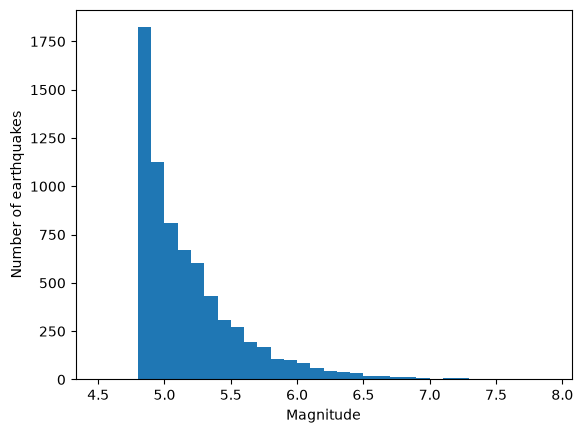
地震震级-频度关系
地震震级-频度关系应符合 Gutenberg–Richter 定律。为了绘制地震震级-频度关系,
首先需要计算得到 GR 定律里的 ,即大于等于某个特定震级 的地震数目。
这里,我们选择 的取值范围为 4.0 到 8.0,间隔为 0.1。计算 的方法有很多,下面的
方法使用了 Python 的列表表达式以及 numpy.sum() 函数来实现:
mw = np.arange(4.0, 8.0, 0.1)
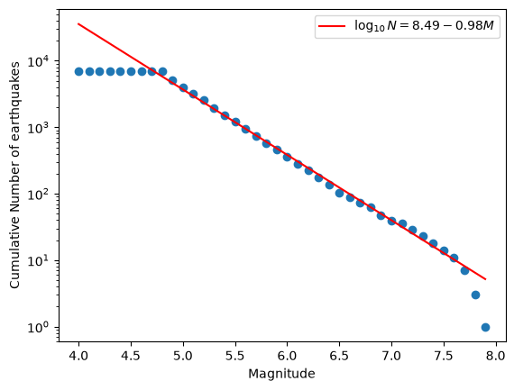
counts = np.array([(mag >= m).sum() for m in mw])绘图脚本如下,注意图中 Y 轴是对数坐标。从图中可以明显看到 与 在 4.8 - 7.6 级 之间存在线性关系。由于我们使用的地震目录里只有 4.8 级以上的地震,所以在 4.7 级以下偏离了线性关系,而大地震由于数目太少也偏离了线性关系。
fig, ax = plt.subplots()
ax.semilogy(mw, counts, "o")
ax.set_xlabel("Magnitude")
ax.set_ylabel("Cumulative Number of earthquakes")
plt.show()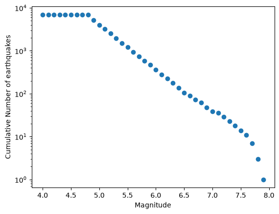
更进一步,我们可以对 4.8-7.6 级之间的数据进行线性拟合,得到 GR 定律中的系数 和 。
这里我们采用 numpy.logical_and 函数找到数组 mw 中所有满足条件的元素的索引,
并使用 NumPy 的布尔索引功能筛选出满足条件的震级 mw[idx] 和对应的 counts[idx],再
使用 numpy.polyfit 函数拟合一元一次多项式,最后绘图:
idx = np.logical_and(mw >= 4.8, mw <= 7.5)
# fitting y = p[0] * x + p[1]
p = np.polyfit(mw[idx], np.log10(counts[idx]), 1)
N_pred = 10 ** (mw * p[0] + p[1])

fig, ax = plt.subplots()
ax.semilogy(mw, counts, "o")
ax.semilogy(mw, N_pred, color="red", label=rf"$\log_{{10}} N={p[1]:.2f}{p[0]:.2f}M$")
ax.legend()
ax.set_xlabel("Magnitude")
ax.set_ylabel("Cumulative Number of earthquakes")
plt.show()